Some of these options can be really useful, such as when you learn how to make a pivot table in Excel 2010. Our Microsoft Excel 2010 pivot table guide below is going to talk a bit about what a pivot table is, when you should use it, and how to create one. Microsoft Excel 2010 users are always looking for the best way to organize and sort the data in their spreadsheets. This can be accomplished in a number of different ways, and your situation will likely be the dictating scenario in determining which method is right for you. However, a pivot table in Microsoft Excel 2010 is an amazing tool for summarizing the data that you have and finding the information that you need. A pivot table is ideal for scenarios where you have a particular item that you want to summarize, like a product or a date, and a secondary set of data that you want to summarize based upon those parameters. Our tutorial on creating tables in Excel provides additional information on using tables in addition to the other tools that you might be using in your spreadsheets.
When Should I Use a Pivot Table?
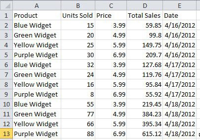
Determining when you should use a pivot table can be tricky, so the first thing to do is figure out what sort of information you are trying to obtain. Ideally a pivot table should be used when the question you are trying to answer is similar to How much of xx did we sell? or How much money did we make selling xx? These are both questions that can be answered if you have a spreadsheet with columns that contain a product column, a units sold column, a price column and a total sales column. There can be other columns as well, but you must have a column containing data for each piece of information that you want to summarize. For example, in the image below, you can see that I have five columns, although I only need data from four of them. I can create a pivot table to summarize the data contained in this spreadsheet, which will prevent me from having to manually determine the answer myself. While it would not be difficult with a small set of data like this, manually summarizing data can be an extremely tedious endeavor when you are dealing with thousands of pieces of data, so a pivot table can literally save hours of work.
How to Create a Pivot Table in Excel (Guide with Pictures)
The steps in this guide were performed in the Excel 2010 version of the application, but will work in most other versions of Microsoft Excel as well.
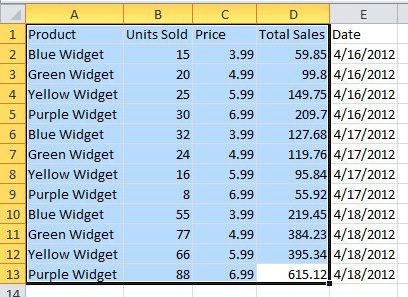
Step 1: Determine which columns contain the data that you want to summarize, then highlight those columns.
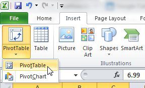
Step 2: When all of your data is selected, click the Insert tab at the top of the window, click the PivotTable icon in the Tables section of the ribbon, then click the PivotTable option.
If you do not know, the ribbon is the horizontal menu bar at the top of the window. The image below shows both the Insert tab and the PivotTable items that you want to click.
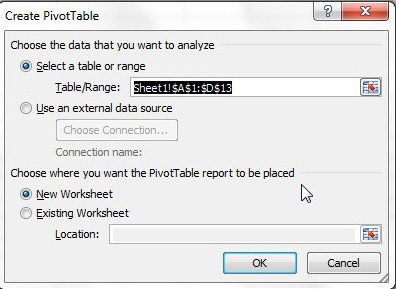
Step 3: This opens a new Create PivotTable window, like the one shown below. All of the information on this window is correct because of the data that you highlighted earlier, so you can just click the OK button.
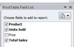
Step 4: Your pivot table will open as a new sheet in the Excel workbook. At the right side of this sheet is a PivotTable Field List column containing the names of the columns that you selected earlier. Check the box to the left of each column name that will be included in the pivot table.
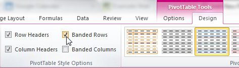
I did not check the Price column because I do not need to display that summarized data in my pivot table. This will change the information shown on the screen so that your completed pivot table is displayed. You will note that all of the data is summarized so, in our example, you can see how much of each product was sold, and the total dollar volume of all of those sales. When you are dealing with a lot of line items, however, reports of this nature can become difficult to read. Therefore, I like to customize my pivot tables a little using the options on the Design tab of the PivotTable Tools section of the ribbon. Click the Design tab at the top of the window to see these options. One way to ease the reading of a pivot table is to check the Banded Rows option in the PivotTable Style Options section of the ribbon. This will alternate the row colors in your pivot table, making the report much easier to read.
Additional Sources
After receiving his Bachelor’s and Master’s degrees in Computer Science he spent several years working in IT management for small businesses. However, he now works full time writing content online and creating websites. His main writing topics include iPhones, Microsoft Office, Google Apps, Android, and Photoshop, but he has also written about many other tech topics as well. Read his full bio here.
You may opt out at any time. Read our Privacy Policy