But one of the more useful things that you can do is learn how to subtract in Excel. Being able to compare data cells with one another and find the difference between them is something that you will find yourself doing, even in more complex formulas and worksheets.
How to Use the Subtraction Formula in Excel
Continue reading below for more information on how to subtract in Excel, as well as view pictures of these steps. Microsoft Excel can do more than just store and sort data. You can also compare data and use mathematical functions. This means it’s possible to add, subtract, divide, and multiply in Excel 2013. You can use combinations of these functions to generate percentage values. if you need to know how to do this, then check out our how to calculate percentage in Excel article. Learning how to use some of the common mathematical operations, like subtraction, in Excel 2013 with a formula will provide you with a gateway into the world of Excel formulas. There are a number of different calculations that Excel is capable of performing, many of which can save you a lot of time if you regularly work with Excel spreadsheets. This article will provide a brief overview of the Excel subtraction formula, plus some examples of that formula that you can apply to your own spreadsheets. Specifically, we will focus on subtracting in Excel 2013 by specifying two cell locations that contain numerical values. You can read our Microsoft Excel tutorial on how to add columns if you’ve been looking for an easy way to generate totals for an entire column of values.
How to Use the Formula for Subtraction Excel 2013 – Subtracting Two Cell Values
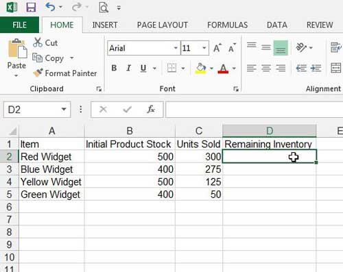
The steps in this tutorial assume that you have a cell containing a value that you want to subtract. You can either subtract this value from a value in another cell, or you can subtract it from a number that you select. This simple formula is very versatile, and we will show you a couple of other ways that you can use it at the end of the article. If you want to subtract a cell value from a number that is not in a cell, simply replace one of your cell locations with that number instead. I am going to display my result in cell D2 in the example below. Excel cells are referred to by their column and row location. So cell D2 is in column D and row 2. For example, the formula =100-B2 would subtract my value in cell B2 from 100. The important thing to remember when you are learning how to subtract in Excel is that subtracting one value from another requires four basic components. While we have specifically learned about Excel subtraction when at least one of the values is a cell location, you can also use the subtraction formula to subtract two numbers. For example, typing “=10-3” will display “7” in the cell, despite the fact that no cell locations were present.
Additional Information on Subtracting Cell Values in Microsoft Excel
Rather than typing the cell references into the subtraction formula, you can click the cells instead. Simply click inside the cell where you want to display the result of the formula, type = into the cell, click the first cell, type – , then click the second cell. Note that the formula bar above the spreadsheet will update as you add each part to this subtract function. If you have a mixture of positive and negative numbers in your cells and want to get a total for all of those values, you can use the SUM function instead. Excel treats numbers with a “-” in front of them as negative, so adding a positive and a negative number together will subtract the negative number from the positive number. For example, if cell A1 had a value of “10” and cell A2 had a value of “-5” then the formula =SUM(A1:A2) would give a total of “5”. When we use cell references in subtraction formulas it is important to remember that Excel is basing its calculations on the values in those cells. If you change a number inside a cell that is being used as part of a formula, that formula will update to reflect the new cell value. The formula is similar if you want to use other common mathematical operations, like addition, division, and multiplication.
How to Subtract Two Numbers in a Cell in Excel
In the sections above we showed you how to subtract in Excel when you had cells that contained values. But what if you want to subtract two numbers in a cell by themselves? The process for achieving that result is very similar to what we learned in the section above. If you type =20-11 into a cell, that cell would display “9”.
How to Subtract a Range of Cells in Excel
While we have focused on subtracting a value of one cell from another cell in the steps above, you can also subtract a lot of cells from a starting value as well. This is accomplished with the help of the SUM function that will add together values in a cell range. In our example we are going to have a value of “20” in cell A1. In cell A2 we have a value of 2, in cell A3 we have a value of 3, and in cell A4 we have a value of 4. If we type the formula =A1-SUM(A2:A4) Excel will display the number 11, which is the result of 20-2-3-4. This can be expanded to incorporate a large number of cells, allowing us to calculate values that include a lot of different pieces of data. For example, if you had 100 numbers in column A that you wanted to subtract from the value in cell A1, you could use the formula =A1-SUM(A2:A101). So the formula for subtracting multiple cells in Excel would look something like =A1-SUM(B1:B5). For example, the formula of =SUM(6+7+8)-5 would display the result of “16” as it is adding the three numbers inside the parentheses, then subtracting 5 from that total. As a refresher, that would be something like =A1-SUM(B1:B100), which would subtract all of the values in the first 100 cells of column B from the first cell in column A. Alternatively, if you wanted to apply the same subtraction formula to an entire column you could type the formula into the top cell, then copy and paste it into the rest of the cells in the column. If you don’t want this to happen, then you can put a $ in front of the values in your formula, which will turn it into an absolute reference. For example, if you had a formula like =d1-b6-2, and you always wanted to use the value in the b6 cell regardless of where the formula was, then you could change it to =d1-$b6-2. Simply click in an empty cell, type something like =12-8 and press Enter on your keyboard. Excel will then display the correct answer in the cell. You can learn more about creating formulas in Excel 2013 if you are ready to start unleashing the potential of your current data. If you need to display the formula instead of the result of the formula, then this article will show you what changes you need to make for that to occur. After receiving his Bachelor’s and Master’s degrees in Computer Science he spent several years working in IT management for small businesses. However, he now works full time writing content online and creating websites. His main writing topics include iPhones, Microsoft Office, Google Apps, Android, and Photoshop, but he has also written about many other tech topics as well. Read his full bio here.
You may opt out at any time. Read our Privacy Policy